Time Resolution in Digital Audio

After having covered the more or less well known basics of digital audio in terms of bit depth and samplerate, I’d like to go one step further and explore another common buzzword: the time domain resolution of digital audio.

If you have read more than one article here, it might have become obvious to you that I am a strong advocate for digital audio technology. Given my profession, this is not surprising. But of course I know about the skepticism that digital audio topics still traditionally provoke. Sometimes of course for good reasons, especially when it comes to actual signal processing. However, one of my goals with The Science of Sound is to promote an informed debate about the advantages and shortcomings of digital audio by helping understand the very foundation of the technology.

One of the concerns about digital audio I frequently encounter is one about the resolution in time domain. In this context, it is often suggested that the precision with which the exact timing of a sound event can be represented is limited to the sampling period. As time differences are a very important feature the ears use to determine sound source direction and spatiality, this coarse resolution must consequently be detrimental to the spatial impression of a sound recording.

Note that for a standard CD sampling rate, the sampling period is around 23 microseconds. And this could indeed be a little too coarse, as hearing studies found that some people are able to reliably identify interaural time differences as low as 15 microseconds for low-frequency sounds. That’s bad news isn’t it?

But you might have already guessed that it’s not that bad in reality. Think about it for a second. How do “sound events” know anything about the sampling period and how would a converter decide how to “quantize” these sound events? In fact, in reality there is no such thing as a sound event, just continuous signals.

Now the sampling theorem states that a signal can be perfectly reconstructed from samples taken at regular intervals, as long as it is bandlimited to half of the sampling rate. That includes any phase information, which – very simply speaking – determines when stuff happens exactly.

A Sub-Sample Time Shift Example

Have a look at this funny little animation here.

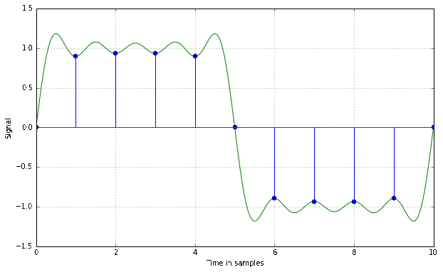
This is a bandlimited version of a square wave period, as an A/D converter would see it after antialias filtering. It is time shifted by different amounts up to one sample. Notice the dots, which represent the actually recorded sample that would land in your .wav file, and observe how they change with the time shift.

This example shows quite well how the sampling theorem actually works. The original signal is the only one possible that contains no frequency components above the Nyquist frequency and still passes through all of the sampled points.

But what about this strange overshoot and the limited steepness of the steps? That doesn’t look like a real square wave. Isn’t that a problem?

Actually not. These phenomena are a direct result of the band limitation. A steeper slope with less overshoot would be equivalent to a larger bandwidth of the signal, which would violate the sampling theorem and cause artifacts. A perfect step function actually has an infinite bandwidth, at no extra benefit in terms of perception, as everything in our hearing range is unaffected by the increased bandwidth. It has to look strange in order to not sound strange!

Time Resolution in Signal Processing

So recording and playback is fine. What about delay effects? Precision of delay is limited to sample steps, right?

Well, only if the developer was lazy. A very simple delay would just shift the audio playback by a number of samples and that’s it. But most implementations will need a process called interpolation. This is important if you need a very precise delay, as for example in physical modeling synthesis, or if you want to change the delay smoothly without artifacts.

Interpolation means computing the reconstructed signal that you would get at the output of a D/A converter at certain time instances between the samples. Thus, the same principle is also used for samplerate conversion. There are several ways to look at it, but in essence, it’s all the same principle. For a precision delay you would combine a sample-precise delay with a filter that adds a sub-sample time shift to the signal and you’re done. However, there are countless different ways to create such a filter, from simple linear interpolation (which has some artifacts but can sometimes be sufficient, depending on the application’s requirements) to a high-end sinc interpolation which will cost a dime or two in terms of CPU load.

Crunching the Numbers

Does that mean time domain precision is actually infinite? It must be limited in some way…

It actually is. But in a practically absolutely neglectable way. Let’s go back a few paragraphs. I wrote that “the original signal is the only one possible that contains no frequency components above the Nyquist frequency and still passes through all of the sampled points”. Now it becomes clear how we can derive the actual time domain resolution: we need to find out by what amount we can shift a signal in time without changing the resulting sample values.

Obviously (?) the limit we will face has to do with the bit depth. The time shift must be large enough for the resulting sample values to change by at least the quantization level, otherwise they would stay the same due to quantization.

I was once even bored enough to calculate that roughly. The result depends a lot on the signal and its level. For a sine signal, the limit gets smaller when frequency and or level is increased. So for a worst case of a 10 Hz sine with -60dBFS magnitude quantized at 24 Bits resolution, we get into a range of around 4 microseconds resolution. Which is already pretty coarse, but you wouldn’t hear that sound anyway. For a more realistic 100 Hz sine at -20 dBFS we are in the range of 4 nanoseconds. By the way, the samplerate doesn’t even show up in the equations!

Although this is a very rough estimate for a very artificial situation, I would suggest that we worry a little less about that in the future. In practice, the actual resolution will be limited by analog noise anyway. However, what we might need to worry about instead is the importance of a good signal to noise ratio – especially at low frequencies – for the spatial impression of a stereo recording!

So it seems like today we’ve pushed another elephant out of the room (but I guess I just let another one in). Soon we should be able to get to the real issues. Stay tuned for more!