Intersample Peaks And Beyond

Intersample peaks are one of those scary phenomena in audio that have been overlooked for a long time, until the awareness about the issue started to spread around the turn of the century. But what if there’s even worse issues with heavily compressed and limited music?

Luckily, the famous loudness war seems to be on a decline recently. With the advent of loudness standards for broadcasting and streaming services and the discovery that music listeners are actually capable of adjusting a volume knob to their own liking, the world is finally becoming a less compressed place. Suddenly it’s possible again to enjoy new releases that actually have some dynamics left in them.

One of the “Oh my god, what have we done?” moments might have been the discovery that 0 dBFS is not the final frontier in digital audio. The existence of intersample peaks means that an analog signal might have peak levels higher than the digital maximum level.

Meanwhile most DAWs are equipped with “true peak” metering and limiting to make sure this doesn’t happen. And generally, there is a trend back towards more headroom and thus less possibility of strong intersample peaks.

The issue of intersample peaks teaches a lesson that the life of digital audio signals doesn’t end after delivering numbers to a D/A converter. And there might be more similar issues that have been overlooked so far.

What are Intersample Peaks Again?

But before we get to it, let’s recap what intersample peaks really are. As the name suggests, the term describes peaks in an audio signal that occur between the samples. A digital system does not “see” these peaks, as they are generated during reconstruction of the analog signal.

It all has to do with the sampling theorem, which says that there is only one possible bandlimited waveform that goes through all the sampled points. The “curve” between two samples is never just a straight line. And most certainly it’s not a stair step.

A good waveform to illustrate this is a square wave where the period length is a multiple of two samples. In this case, we have neither aliasing nor overshoot in the digital domain, but the overshoot will become visible in the analog domain.

Have a close look at this zoomed-in picture of such a waveform:

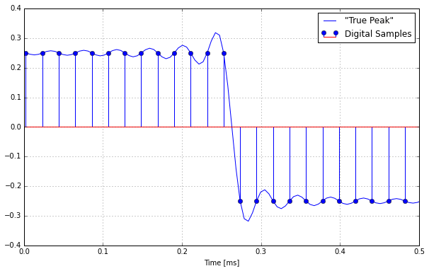
The dots depict the actual digital samples, the second curve shows a 4x oversampled version of the same signal. Oversampling is the usual method to detect intersample peaks in the analog domain. Read this great article by the good guys at iZotope for more info on that.

You see that there is a significant overshoot of the oversampled signal. The same happens in the analog domain upon reconstruction.

What’s The Problem With Intersample Peaks?

Intersample peaks create several problems. The explanation you’ll see the most out there is that the overshoots exceed the headroom of the analog circuitry that follows the actual D/A converter and thus lead to clipping distortion. That can certainly be true if the converter is tightly dimensioned.

Additionally, problems can also occur right inside the D/A converter. Most converters used today are so-called delta-sigma converters which internally convert the audio into a heavily oversampled 1-Bit signal. I won’t go into detail today, but this method can react quite nastily to overloads during signal processing.

A third problem is lossy compression formats which deconstruct and process audio so that digital clipping can occur during encoding. This can also be much worse than clipping in the analog domain.

But let’s look a bit further into the analog domain and see what else can happen there in terms of peak levels.

Another Type of “Invisible” Peaks

If we are worried about intersample peaks, there is another issue that we should be aware of. As mentioned before, the lifetime of a signal doesn’t end when digital data is transmitted to the converter. But it also doesn’t end at the output of the converter.

After leaving the converter as a hopefully near-perfect reconstruction of an analog signal in accordance with the sampling theorem, audio signals pass several more electronic circuits. In a mastering studio setting, this might just be a monitor controller and a power amplifier. A recording studio might have a whole console signal path in between the converter and the speakers. In domestic consumer audio systems, there might be all kinds of preamps, EQs, “loudness” circuits and so on.

Even in the most puristic setup, there will be some circuitry, which in practice is most likely coupled to the following devices via coupling capacitors to filter out any DC offsets. Either at an output stage, an input stage, or very likely both. This essentially presents a highpass filter with very low cutoff frequency.

The case is similar for high frequencies. Audio devices usually limit their frequency range deliberately by lowpass filters to improve noise performance and reduce susceptibility to high-frequency interference, intermodulation and parasitic oscillation.

These filters have cutoff frequencies set so that their effect in the audible range is as small as possible. An indeed, if everything is perfectly linear, these things are practically inaudible.

However, the effect of such circuitry on phase response can extend much further than around the cutoff frequencies. And as we’ve learned already, phase determines the distribution of energy over time.

An Example

Let’s look at what happens to our 100 Hz square wave from above when it passes a 12 dB/oct highpass filter at 30 Hz.

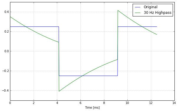
The filter cuts off low enough to not audibly affect the magnitudes of the square wave. It doesn’t take away any energy from the signal. Still the waveform changes drastically.

The original square wave has its signal energy distributed equally over time. The filter changes that. It takes away energy from some regions and puts it somewhere else. The RMS level stays the same, but peak level increases strongly.

In Numbers

So let’s look at the numbers for this artificial example.

The original square wave has a peak level of -12.04 dBFS, while the true (intersample) peak level is at -9.94 dBFS, an increase of 2.1 dB.

The digital peak level of the highpass filtered signal reaches -7.62 dBFS, with a true peak level of -6.32 dBFS. Thus, the true peak of this highpass-filtered analog signal is nearly 6 dB higher than the original digital peak level, thus nearly double the voltage!

Conclusion

Of course this is an artificial example, and that doesn’t have much significance in practice. In the real world, the peak level increase will be smaller, but still significant.

You can easily test it for yourself with real world material. Just take some of your own material or something from your music library, put some low-cutoff highpass filters on it and notice the increase of peak levels. Also compare with readings of true peak meters to put things into perspective. In my own tests, with loudly mastered music, the effects of highpass filtering have been consistently stronger than the difference in peak level due to intersample peaks alone.

So this is another good reason to continue the trend towards softer and more dynamic masters. With more air to breathe, such nifty phenomena won’t destroy our listening pleasure.

Have you tested this issue with some of your favorite tracks? Share your results in the comments!