
Sound Localization Basics
Creating an illusion of space is a key element of music and sound design. But to be convincing, we need to understand the mechanisms of spatial hearing. The most important component of that is sound localization.
As you might have found out already, I’m constantly amazed by everything regarding human hearing. The elegance and efficiency with which an enormous amount of information is extracted from the sound field is really stunning. Today I’d like to walk you through the strategies of human hearing to determine from which direction a sound is coming.
This is only a small part of spatial hearing though. There are much more mechanisms in play to reduce noise and reverberation or estimate sound source distance or the geometry of the acoustic environment. However, today I’ll focus on sound localization.
Sound Localization
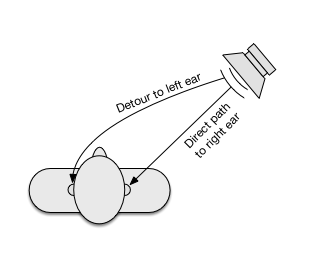
The most prominent strategy to estimate sound source direction is of course binaural hearing. The term refers to evaluating differences between the signals arriving at both ears. These differences are in level and time of arrival. Here’s a little illustration:
One important thing to realize is that this strategy only works in the horizontal plane, because the vertical direction of a sound source doesn’t result in large interaural differences. So for the vertical direction we have to rely on monaural cues, which affect both ear signals similarly.
As a result, the precision with which source directions can be distinguished is much finer in the horizontal plane. Humans can usually distinguish source displacements of down to 1° in the horizontal plane, while perception of vertical displacement is more in the 5° range at best.
Let’s have a closer look at interaural differences first.
Interaural Level Differences
If you look at the above picture, you see that there is no straight line from the loudspeaker to the left ear. The head creates a kind of shadow that leads to sound at the left ear being damped a bit. The maximum level difference – when the sound source is at the extreme left or right – is around 20 dB.
So far, so obvious. Chances are you knew that already, as it’s kind of common sense. But there’s a little more to it, which is often forgotten. The head shadowing effect only works at high frequencies. At lower frequencies, when the wavelengths of sound are in the range of the head diameter, this doesn’t work anymore. In this range lower than 700-800 Hz, the head presents no significant obstacle to the sound waves. They just “bend” around it.
As a result, there are typically no interaural level differences in the lower frequency range. Head shadowing works to its full extent only above 1400-1600 Hz.
That’s for sounds occuring naturally in the sound field though. Level-based sound localization does still work at lower frequencies when created artificially (via a pan pot for example).
Interaural Time Differences
As is obvious from the illustration above, sound also takes a bit longer to take the detour (up to 0.5-1 ms) around the head. This difference in time of arrival is thus also used to determine source direction. To do that, the auditory system evaluates phase differences between the two ear signals.
But here again, the head geometry plays an important role. This also has to do with the relation between head diameter and sound wavelength. And interestingly, we encounter the same frequency limits as before.
Above 700 Hz, the phase difference between both ears becomes ambiguous. That means the same phase shift could be caused by a source displacement to the left or to the right. Double the limit, and above 1400 Hz there could even be three or more possible source directions that lead to a certain phase difference.
Up to 1400 Hz, the auditory system uses a simple trick to decide between the two possible directions. In that range, level differences start to occur, and so the decision is made for the side where the signal is louder.
Now that’s for pure sine tones. For more complex signals, the envelope modulation can also play a role. So time-based sound localization is possible for higher frequency content. But it’s not as effective and accurate as the phase-based localization at low frequencies.
At this point, I encourage you to play around and try it out for yourself. With a sine oscillator, a very short stereo delay and a pan pot you can create the cues and test your perception at different frequencies. With a tremolo or a rather fast synth envelope, you can also test time-based localization at high frequencies.
Spectral Cues
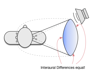
I already mentioned above that interaural differences are only really useful in the horizontal plane. For vertical displacement, interaural level and time differences don’t vary much. The phenomenon is called the “cone of confusion”, because the source directions that result in the same interaural differences lie on a cone, as depicted in the image below.
Nevertheless, we are able to distinguish source direction on this cone of confusion to some extent, although not as accurate. The way that works is by evaluating spectral properties of the signal.
In order for that to work, the signal needs to have a rather broad spectrum. With steady sine waves we get confused very easily.
The tool that enables this kind of processing is the outer ear. Its several cavities create specific resonances, but with a nice additional feature: the resonances get excited to a different extent depending on sound source direction. So when certain resonances are prominent, the sound was likely emitted from the direction that most strongly excites these resonances.
The exact pinna resonances vary for different people. Each of us is used to his personal resonance profile which makes this sound localization strategy work. But even though there’s quite some variation, there are some frequency bands that are common to a majority of people.
This takes us right back to the very beginning of The Science of Sound. On day one, I posted this article that explains these so-called Blauert bands. It’s also kind of the manual for the nice freebie you get when you sign up for my weekly newsletter. The Audio Unit plugin “Jens” let’s you play around with these typical resonances to create an illusion of front/back localization and elevation. If you haven’t yet, sign up and try it out!
Conclusions
As you can see, there are several strategies combined to estimate sound source direction. In real life, this is very effective.
To a certain extent, it is possible to create these features used for sound localization artificially. But the individual variability and practical issues as well as conflicting requirements make it hard to create the ultimate spatial illusion.
For example, the possibilities to create artificial sound localization cues using stereo loudspeakers are quite limited. Also, mono compatibility is sometimes also desired, especially in music. Artificial time difference cues can lead to problems like comb filtering when mixed to mono. Finally, accurate reproduction of spectral cues requires knowledge of the listener’s individual profile and is likely to sound colored.
Have you used advanced spatialization techniques beyond panning? Share your experiences in the comments!