
Oversampling In Digital Equalizers
We continue our tour through signal-processing algorithms that benefit from high sampling rates. This time we’ll look at what the oversampling option that can be found in many digital equalizer plugins does.
Most of the time you’ll encounter very simplistic explanations when it comes to the question why high sampling rates would be beneficial. It usually goes along the lines of “well, it’s just more analog!”. So as long as the “analogness” of something is the ultimate criterion, we can keep discussion short and simple.
But with The Science of Sound being the temple of the slightly longer and more complicated explanation, let’s have a closer look at the effects of oversampling in digital equalizers.
Oversampling Equalizers
Last week we looked at oversampling in the context of nonlinear distortion effects. In that case, oversampling is primarily a means for reducing nasty aliasing artifacts. With the purely linear processing found in digital equalizers, we don’t have that kind of artifacts.
Linear processing does not introduce any new signal components like nonlinear processing does. It only affects the frequency response of the signals that are there already.
That said, we don’t need oversampling in equalizers as desperately as in distortion effects. But anyway, it can still yield some nice benefits.
An interesting thing is that with distortion effects, oversampling is usually happening largely unnoticed by the user. Under the hood, so to say, as a fixed part of the DSP algorithm.
With digital equalizers, there is often an explicit option for the user to choose the amount of oversampling to his liking. That’s a bit surprising, because in both cases, the amount of oversampling that is really needed depends on a couple of parameters.
However, the result is that it triggers the user’s sense for “bigger is better”. Surely, an oversampling EQ must be better than a normal one. And the more oversampling I engage, the better the sound will be, right?
Let’s look at what happens exactly.
Typical EQ Filters
First we have to take a look at what’s inside an equalizer actually. Practically all of the typical modern parametric equalizers consist of a couple of so-called second order IIR filters. The beautiful thing about these is that they are extremely versatile and you can split any complex linear system up into a series or parallel combination of these filters.
With a second order filter structure you can implement the three basic filter shapes lowpass, highpass and bandpass. Or any combination of these which result in the also well-known shelving, peaking or notch filter shapes, and the more exotic allpass filter. All this with one simple filter structure.
Digital Filter Design
The above catalog of filter prototypes was originally defined in the analog domain. And by analog I mean the abstract theoretical concept of dealing with continuous signals.
In the analog domain, a second order filter is defined by a differential equation. Whereas in the digital domain, we deal with so-called difference equations.
The former consists of some additions, multiplications and differentiators (or integrators) that compute the derivative or integral of a signal. A second order filter in digital domain looks very similar, with the exception that instead of differentiators or integrators, there are delay elements.
The structures are very similar, and so are the maths in each domain. In both cases, the behavior is fully defined just by a couple of coefficients. Five of them to be precise.
Bilinear Transform
The challenge in digital filter design is to properly convert the analog coefficients into the digital ones so that the frequency response is retained as best as possible.
The widespread – although not the only – method to achieve this is the bilinear transform. It’s so popular because it retains some important properties of the analog filter, such as stability, overall filter shape, and the relation between magnitude and phase response.
But unfortunately, it has one major drawback:
Frequency Warping
The bilinear transform retains the overall filter shape of the analog filter by squeezing its whole frequency range (which goes from 0Hz to infinity) into the limited digital frequency range from 0 Hz to half of the sampling rate (the Nyquist limit). Sounds brutal, right?
It is. And added to that, the “amount” of squeezing is frequency dependent. The higher the frequency, the more the frequency response is squeezed.
The warping has only a slight effect at low frequencies up to 1/4 of the Nyquist frequency. So in typical audio scenarios, it starts to kick in above around 5 kHz. It’s most extreme towards the Nyquist limit.
The only compensation that is usually applied is to change the cutoff or center frequency of the original filter in such a way that it lands at the right frequency after warping. But that only alleviates a small bit of the pain.
Here’s an example to illustrate what that happens. We specify a combination of a highpass filter at 100 Hz and a resonant lowpass filter at 15 kHz, and create a digital implementation at a sampling rate of 44.1 kHz. Here are the frequency responses of the analog original and the warped digital version, with a compensation of cutoff frequencies:
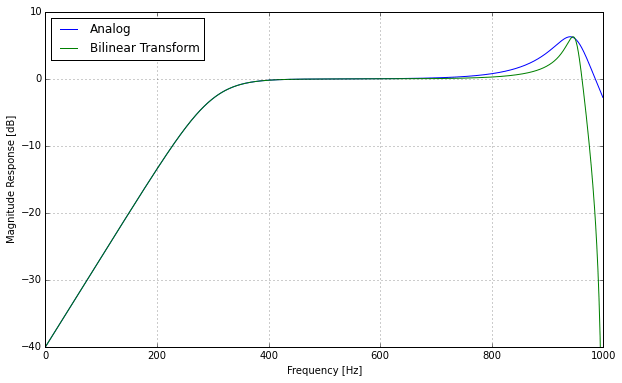
The highpass filter doesn’t change at all because it affects only the low unwarped frequency range. But the lowpass filter suffers quite a bit from the bilinear transform. The resonance peak is narrower and the lowpass slope isn’t as straight as the original one. It deviates quite a bit towards high frequencies and goes all the way down to infinite damping at the Nyquist limit.
Oversampling
Apart from using other transform strategies, each with their own set of unique ins and outs, a convenient way to reduce this effect and get closer to the response of the originally specified analog filter is – of course – oversampling.
As we know that the warping starts to kick in at 1/4 of the Nyquist limit, a reasonable choice would be an oversampling factor of 4x. And obviously, if the EQ setting does not affect frequencies higher than around 5 kHz, oversampling won’t make much of a difference. So the highest frequency your EQ setting affects is a good criterion to choose an appropriate oversampling factor by.
Conclusions
So this is how oversampling affects the response of digital equalizers. Note again that this is not about nasty artifacts, but about a change of the behavior of digital equalizers.
I wouldn’t describe the phenomenon as a matter of audio quality. It’s rather in the realm of taste or finding the best tool for the job. It depends on what you are trying to achieve with an equalizer if you need oversampling or if you’re ok with the response that the normal digital filter provides.
But on the other hand, it possibly explains digital filter’s reputation of sounding a bit harsh compared to their analog counterparts. Peak filters especially become narrower at high center frequencies. In other words, their Q factor becomes larger and the slopes a bit asymmetric.
Oversampling in the EQ itself is one solution. Running the whole session at high sampling rates is another one. So this is one of the possible reasons why many people like to work at such rates.
I personally wouldn’t bother wasting so much CPU and instead make sure I use (and develop) processing tools that work as I intend them to do, with the necessary measures taken where it matters, not blindly all over the place.
And in many cases it might even be sufficient to just use lower Q factors at high frequencies.
Are you using oversampling equalizers regularly? What effect have you observed when working with them? Share your experience in the comments!