Zero-Delay Feedback vs. Oversampling

In the third part of the oversampling series, we look at a case where oversampling is not necessarily the best answer. At the same time, we get a first glimpse at what all the “zero-delay feedback” fuss is about.

The recurring topic of the last two weeks has been signal processing algorithms that collide in one way or another with the constraints that digital signal processing and especially the choice of sampling rate imposes on them. For both distortion effects and digital filters, oversampling is an effective way of minimizing unwanted artifacts or increasing accuracy compared to analog signal processing.

Today I’d like to look at algorithms that encounter similar limitations at normal sampling rates, and that benefit from oversampling in a similar way. However, in this case, blindly increasing the sampling rate is not the only solution, and it’s also not the best one. I’m talking about analog modeling.

What is Analog Modeling?

Unfortunately, analog modeling has been a preferred playground in the past for marketing people. Thus there are a lot of three-lettered technology trademarks out there that are usually designed to make you think that every single electron inside the good old Fairchild is simulated to perfection. Or maybe at least down to component-level.

I’m pretty sure nobody ever really does this to full extent. It would be like admitting you haven’t understood at all what’s special about the device in question and thus resorted to blindly simulating a schematic (and thus wasting your customer’s precious cpu performance).

But I digress. The process of analog modeling is about figuring out a mathematical description of how an electric circuit behaves and then modifying it until it’s implementable digitally. That’s true, you need to mess around with the accurate mathematical model quite a bit in order to get something that you can actually work with. That means, leaving stuff out, approximating stuff, or moving stuff to a place where it doesn’t hurt your lower back so much.

These compromises aren’t just a matter of mere computational power. They’re also a means of better understanding the system in question, and finding gimmicks, improvements and possibilities that might make the simulation bigger and better than the original.

However, the main point here is that it’s all about mathematical models, not about just connecting individual simulated components, which would be a highly impractical solution to the problem.

The Zero-Delay Feedback Problem

With these mathematical models, it’s often useful to visualize them as block diagrams in order to get a good overview on what’s happening. Here’s an example block diagram that shows a model of a one-pole lowpass filter based on an operational transconductance amplifier (OTA). Many 4-pole synthesizer VCFs are built around this basic structure.

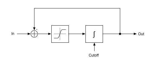
Simple Nonlinear One-Pole Lowpass Filter Model

The most important part is the integrator, which is the rightmost of the two boxes. In the actual circuit, this integrator consists the OTA output in conjunction with a capacitor and an additional buffer amplifier stage.

Note that before the integrator, there’s also a distortion element that represents the nonlinear characteristics of the OTA’s input stage. This one is what makes the filter really interesting. And complicated.

But the most important thing here is the fact that the output of this whole model is routed directly back to the input. This feedback is what actually makes this a lowpass filter. Such structures containing some kind of feedback can be found all over audio electronics. And they’re the main reason why translating these models into something that can be computed digitally is tricky.

The thing is that this feedback path creates a loop in this block diagram. The output signal needs to be known in order to compute the output signal.

Wait, what? That’s impossible!

I know this sounds strange. But physics don’t work the same way that our pocket calculator-conditioned brains do. There’s just an equation that unfortunately isn’t resolvable to the output signal easily. But that doesn’t mean a solution doesn’t exist. The output signal is just the one signal that satisfies this equation.

Cheating

Now what can we do to circumvent this problem? As said before, we need to modify the model so we can get something out of it.

The easiest cheat we can apply is to remove the nonlinear element from the model. If there is no nonlinearity, the equations become much simpler. As a result, we can compute the output signal directly.

But we lose the nice distortion of the original system when driven hard. We can cheat some distortion back into the emulation by putting it before or after the filter. However, that will add distortion, but behave completely different to the original. This is probably best described as the 90’s solution.

Let’s try another cheat, and let’s call it the 2000’s solution. The problem being the feedback loop, we could solve it by inserting a tiny delay into the loop so we can compute it. The tiniest delay we can use is one sample in our digital system.

This indeed works up to a certain extent, but with the feedback being always one sample too late, it takes the simulation at least one sample of time to reach the state it would reach in the analog system. The problem is, during that time the input signal has also changed, especially if it has much high-frequency content.

As a result, the simulated system may have problems with stability, and also with accuracy of high-frequency content. The result is harsh and brittle sound, especially with fast modulation. That is, if it doesn’t blow up due to instability in the first place.

But as these problems are caused by the additional delay inside the feedback loop, we could try to make the delay smaller so it has less effect and works “faster”. Simply by increasing the sampling rate. Theoretically, if we increase the sampling rate infinitely, we’ll get a perfect simulation.

This does indeed improve things, and in some cases, it’s a viable solution. But is this the best solution?

Enter: Zero-Delay Feedback

You guessed it, it’s probably not. Although we can make such an implementation better and better the more we increase sampling rate, we also waste more and more CPU. At some point, the improvement in sound quality with every further increase of sampling rate becomes quite small, while CPU load explodes.

So let’s go on with the 2010’s solution. Over the last couple of years, several methods have evolved that aim at getting rid of the cheated delay in the feedback. These techniques are often coined as “zero-delay feedback”, also that might not be a completely precise description.

What this does is taking the system equations that don’t have a direct solution and perform an iterative process until a solution is found that satisfies the equation. It’s a bit like starting with a guess, checking the result, and improving the guess over and over.

This yields an almost perfect simulation of the analog system. But as you might have guessed, you have to compute some heavy nonlinear equations over and over until you get to the solution. So that’s quite expensive computationally.

The thing is, it does pay off in the end. The instantaneous feedback is implemented directly and thus there are no stability problems from delayed feedback. And modulation at audio rate is also possible. You’d need extreme amounts of oversampling to get in a similar ballpark of quality.

It should be noted however, that the issues like aliasing and frequency warping still exist also with these zero-delay feedback methods. So it’s still a good idea to add moderate amounts of oversampling. But that doesn’t require as much oversampling as naive methods to achieve competitive quality.

Conclusions

Anytime we encounter limits of digital signal processing due to the choice of sampling rate, oversampling is a way to extend these limits. But just blindly increasing sampling rate is sometimes not the most effective and efficient method.

The instantaneous feedback loops that most electronic audio circuits consist of make a straightforward approach of modeling individual components and connecting them impossible. The circuit must be viewed as a whole.

So-called Zero-Delay Feedback methods do this and solve the modeling problem much more exactly.

I could only barely scratch the surface of this interesting topic here. If you want to know more, you should definitely have a look at Urs Heckmann’s blog. With u-he’s Diva synthesizer, he was significantly involved in paving the way for extremely CPU-hungry, but also extremely accurate analog modeling.

And this most probably wasn’t the last article on The Science of Sound about this exciting topic!